datahandling2

Home

About

Methods

Studies

Themes

Data Handling and Inferential Statistics

This is the page that you will need if you want to make "inferences" about your data. For example, do you have two sets of data that are statistically different from each other? Do you have two sets of data that are statistically significantly related? To find these answers, you will need to carry out one of the tests listed below:
The Wilcoxon Matched Pairs Signed Rank Test
The Mann-Whitney Test
The Wilcoxon Rank Sum Test
Spearman's Rank Correlation Coefficient
The t-test - there are assumptions to make to use this test (see later)

All of these tests assume that you have, at least, ordinal data. The t-test requires interval or ratio level data.

The other thing to note is that I will refer to a value from a table. The tables are from the back of most books about statistics. You have to make sure that you know what table to use and what that value you get, means.

So. let's start!

The Wilcoxon Matched Pairs Signed Rank Test.

This test uses, at least, ordinal data. The experimental design would be matched pairs or repeated measures.

Let's look at an example:
I got 15 students to watch short video clips. One was of a romantic nature, the other was a clip from a reality T.V. show, and I asked them to rate each clip out of a total of 50. The data is below:

Student	Rating of Romantic Film (A)	Rating of Reality T.V. (B)	Difference (B-A)	Rank of Difference
1	23	33	10	12
2	14	22	8	9.5
3	35	38	3	3
4	26	30	4	5
5	28	31	3	3
6	19	17	-2	1
7	42	42	0
8	30	25	-5	6
9	26	34	8	9.5
10	31	24	-7	8
11	18	21	3	3
12	26	46	20	14
13	23	29	6	7
14	31	40	9	11
15	30	41	11	13

You will find that I like to use tables, I find it easier to keep a track of the numbers that I am using.
You will find that one of the students gave the same value to both film clip and therefore the difference was zero. This can be ignored, but you then have to realise that you have lost a data item.
Rank on the basis of absolute value, therefore after 4 comes -5 followed by 6 and so on.
The next thing to do is to add up all the positive rankings and all of the negative rankings, and they are:
The Total Sum of Positive Ranks = 90, n=11
The Total Sum of Negative Ranks = 15, n=3
To find out if there is any significant difference between the two sets of data take the smaller value (T) and remember that the number of students (Sample Size) in the smaller sample =3 and the larger value =11

At some point, it might as well be now, it might be worth thinking about an hypothesis. The total rating for each film clip are as follows: ratings for romantic film totaled 402, ratings for Reality TV totaled 473. So generally, people like the reality TV clip more, and rated it higher.
So, our Experimental Hypothesis might be that "There will be a significant difference between the rating of the romantic clip and the reality TV clip."
Our Null Hypothesis will be that "There will not be a significant difference between the rating of the romantic clip and the reality TV clip.
Consulting with the appropriate table and using the correct values, our difference does not reach significance, so we reject the Experimental Hypothesis and accept the Null Hypothesis.

The Mann Whitney Test

This is the test you would use to find the difference between two sets of data. For example, I gave 20 people a small Lego model to assemble. All of the models were the same, and they were given 30 second to read the instructions and the time started when they touched the first block. I was fortunate that within my sample of 20 people there were 10 females and 10 males. The time taken to assemble the model is given below:

Males (sec)	Rank	Females (sec)	Rank
20	7.5	18	2
21	9.5	25	18.5
25	18.5	19	5
19	5	20	7.5
18	2	21	9.5
22	11.5	25	18.5
23	13	24	15
24	15	22	11.5
25	18.5	19	5
24	15	18	2

When you rank the times, as here, you will need to rank the time as one big sample, the male and female times together. Then you need to put the values in the table and total the male and females ranks, as here:
Total Sum of Ranks Males = 115.5
Total Sum of Ranks Females = 94.5

Then you need to calculate the value of U.
The formula is: Umales = Nmales x Nfemales +(Nmales(Nfemales + 1)) /2 - Rmales and similar for females.
So, Umales = 10 x 10 + (10(11)) /2 -115.5
Umales = 100+55-115.5
Umales = 39.5
To be significant the calculated U value has to be less than the critical value (27), so there is no significant difference between males and females in the times taken to assemble a Lego model.
Just so you know, I did the same calculation for the females, and it still was not significant.

Wilcoxon Rank Sum Test

This test also looks for a significant difference between two sets of data. Generally, it follows the first part of the Mann Whitney test above, but stop when you have found the two values for the Sum of Ranks. You take the smaller sum and call that "T" and look up in the table for the critical value. The critical value for sample sizes 10 and 10 is 78 and our calculated value is 94.5. To be significant, our calculated T must be equal to or less than, which it is not. So confirmation then, there is no difference in the times that males and females can asssemble a small Lego Model.

Spearman's Rank Correlation Coefficient.

The first thing to discuss is, what is a correlation? A correlation is the extent to which two sets of data relate to each other. A correlation can be positive, as one variable increases, so does the other. For example:
"The further you walk, the more money you collect for charity," and
"The more papers you have to deliver, the longer it takes you."
A correlation can be negative, as one variable increases, the other variable decreases. For example:
"As the temperature increases, the sales of woolly jumpers decrease," and
"The more groceries that you carry, the slower you walk."
Once you have worked out what you are going to study, you have to work out how to measure your variables and how you are going to describe them in an hypothesis. This process is referred to as operationalising your variables.
So here is an example, the thing with correlations is that there has to be a relationship between the sets of data so the design of the study should be repeated measures or matched pairs.
So let us work an example:
We are going to investigate if students who are good at maths are also good at music. This looks like a positive correlation, so our hypothesis should be: There will be a significant relationship between a sample of student's maths and music scores. So here's our data:

Student	Maths Mark	Music Mark	Maths Rank	Music Rank	Difference (d)	d squared
John	53	34	5	2	3	9
Julia	91	43	7	3	4	16
Jerry	49	73	4	5	-1	1
Jean	45	75	3	6	-3	9
Jill	38	93	2	7	-5	25
Jonah	17	18	1	1	0	0
Jasmine	58	71	6	4	2	4

The sum of the differences squared = 64.

The formula is 1- (6 x sum of the difference squared)/n(nsquared - 1)

Spearman = 1- (6 x 64)/ 7(49-1)
Spearman = 1-(384)/336
Spearman = 1-1.143 = -0.143

Correlation values vary between 1 and -1. Our value is close to zero and negative. This means that there is a slight negative correlation between student's ability on maths and music. The critical value for sample size 7 is 0.786. To be significant, our calculated value must be bigger than the critacl value, which it isn't. That means there is no carrelation.
What if there had been a strong correlation between the two sets of marks? What would that mean? Would it be that people who are good at maths are also good at music? Well, yes, that is what we have found, but try and think what these two sets of marks are measuring and what ties them together? Of course, people who are good at stuff are usually more intelligent than people who are not so good. And that is what to think of when you find a strong correlation. Is there something that relates the two sets of variables, that has not been measured?
Think about this situation, when a fire breaks out and has been put out by the fire brigade, the insurance company will set a value of the cost of repair. So that is one set of the variables, the cost of repair. The insurance loss adjuster (or whatever the person is called) noted the number of fire engines that attended each blaze. His son studied statistics at University and found that the cost of repairs after a fire and the number of fire trucks that were sent were strongly positively related. That did not mean that the Fire Chief could bump up the costs of repairs by sending more fire trucks. The fact that these two things are positively related is because they are both positively related to the size and ferocity of the fire.

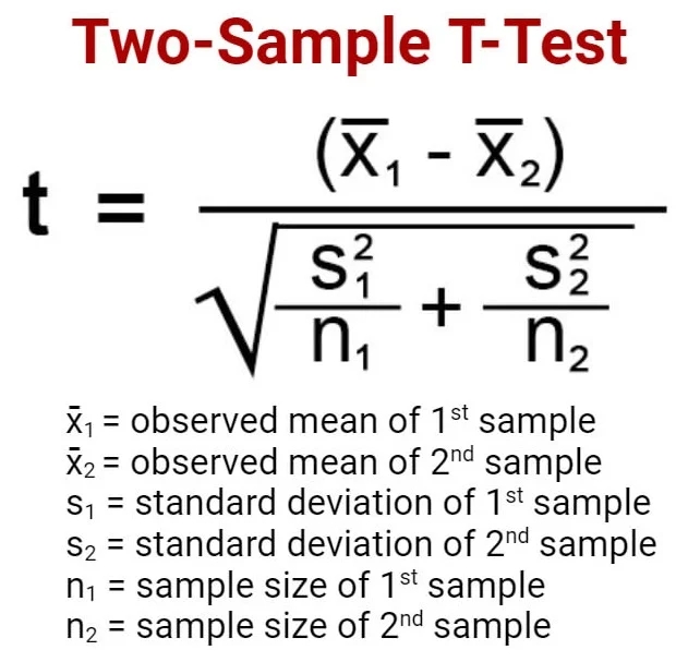
t-test

As I mentioned above, t-tests will only work with at least interval data, and the sample should be drawn from a normally distributed populations. I would think that most of the time you would be reseaarching people, and, as long as your sample is large enough, then it is safe to assume that it satifies this assumption. Anyway, let's get on with an example. You remember that in Loftus and Palmer there was a difference observed in their spped estimates and whether they saw broken glass when participants heard "smashed" or "hit. Loftus and Palmer then went on to measure the probability of participants saying "Yes" to the question about broken glass was also affected by the verb they heard. The table of results looked like this:

P(Y) the probability to "did you see broken glass?", separated on speed estimates
	Speed estimate (m.p.h.)
Verb Condition	1-5	6-10	11-15	16-20
Smashed	0.09	0.27	0.41	0.62
Hit	0.06	0.09	0.23	0.50

This table shows the probability that the participant saw broken glass when asked and also heard the verb "smashed" or "hit" and separated out by speed of estimate. The question I want to ask are those two sets of probabilities different from each other? The number of participants in each group was 50. A clearer view would be if I rearranged the data:

Speed	Smashed	(d)	(d)^2	Hit	(d)	(d)^2
1-5	0.09	0.0622	0.0039	0.06	0.0424	0.0018
6-10	0.27	0.2422	0.0587	0.09	0.0724	0.0052
11-15	0.41	0.3822	0.1461	0.23	0.2124	0.0451
16-20	0.62	0.5922	0.3507	0.50	0.4824	0.2327
Totals	1.39	1.2788	0.5593	0.88	0.8096	0,2849

(d) = the difference between the value and the mean. (d)^2 = (d) squared.

The method that I will use to calculate the value of "t" is:

You may remember that I told you about the variance of a sample and the standard deviation being the square root of the variance. To find "t", which will tell us if the samples are significally different, you will need to find the standard deviation of both samples.
The standard deviation is the square root of the total of the differences squared ((d)^2) divided by the sample size, which is 50.
Standard deviation of "smashed" = the square root of the total of (d)^2 divided by 50.
Standard deviation of "smashed = the square root of 0.5593/50
Standard deviation of "smashed = 0.1058
Similarly,
Standard deviation of "hit" = the square root of the total of (d)^2 divided by 50
Standard deviation of "hit" = the square root of 0.2849/50
Standard deviation of "hit" = 0.0755
To find "t" you need to find the differences between the means divided by the square root of the standard deviation of both samples divided by the sample size.
The difference between the means = 0.0278 - 0.0176 = 0.0102
The standard deviation of "smashed" / 50 = 0.1058/50 = 0.0022
The standard deviation of "hit"/50 = 0.0755/50 = 0.0151
The method to calculate t using the above information = 0.0102/ square root of 0.0022 + 0.0151.
t= 0.0102/0.1315
t = 0.0776
The critical value for t for sample size 50 is, 2.000
To be significant our calculated value of 0.0776 does not exceed the critical value of 2.000, therfore there is no significant difference between the parobability of seeing broken glass for those that heard "smashed" and those that heard "hit"